One sample z-test in R with Examples

In this article, we will discuss how to do a one sample z-test in R with some practical examples.

What is One-sample z-test for mean?

A one-sample z-test is used to determine whether the population mean is equal or different from a predefined standard (or theoretical) value of mean when population standard deviation is known and the sample size is larger.

Conditions required to conduct a one-sample z-test for mean

Assumptions for One Sample z-test for mean

• The parent population from which the sample is drawn should be normal.
• The sample observations should be independent of each other i.e sample should be random.
• The population standard deviation is known.
• The sample size should be larger i.e n>30 at least.

Hypothesis for the one sample z-test for mean

Let μ₀ denote the hypothesized value for the mean and x̄ denotes the sample mean.

Null Hypothesis:

H₀ : x̄= μ₀  The population means is equal to hypothesized mean.

Alternative Hypothesis: Three forms of alternative hypothesis are as follows:

• H_a : x̄< μ₀  Population mean is less than the hypothesized mean.It is called lower tail test (left-tailed test).
• H_a : x̄>μ₀ Population mean is greater than the hypothesized mean.It is called Upper tail test(right-tailed test).
• H_a : x̄ ≠μ₀ Population mean is not equal to hypothesized mean.It is called two tail test.

Formula for the test statistic of one sample z- test for mean is:

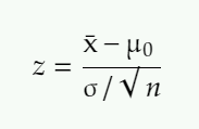
where :

x̄: observed sample mean

μ₀: hypothesized population mean

n: sample size

σ: population standard deviation

Function in R for z-test

z.test() function in R from the BSDA library is used to perform a one-sample z-test for mean.

Install BSDA for z-test for mean

If you don’t have the BSDA library installed then use the below command on the R Editor for BSDA library installation

install.packages("BSDA")

The z.test() function uses the following basic syntax:

z.test(x,y = NULL,
alternative = "two.sided"or"greater", "less" or
mu = 0,
sigma.x = NULL,
sigma.y = NULL,
conf.level = 0.95
)

where :

x,y: given sample data. y will be NULL if only one sample is given.

alternative: The alternative hypothesis for the test. It can be ‘greater’, ‘less’, ‘two. sided’ based on the alternative hypothesis.

mu: The true value of the mean.

sigma.x: It represents the population standard deviation for the x sample.

sigma.y: It represents the population standard deviation for the y sample.

conf. level: confidence level of the interval

Summary for the one sample z-test for mean

	Left-tailed Test	Right-tailed Test	Two-tailed Test
Null Hypothesis	H0 : x̄≥ μ0	H0 : x̄≤ μ0	H0 : x̄= μ0
Alternate Hypothesis	Ha : x̄< μ0	Ha : x̄> μ0	Ha : x̄ ≠ μ0
Test Statistic	z= (x̄ – μ0 )/(σ/ √ n)	z= (x̄ – μ0 )/(σ/ √ n)	z= (x̄ – μ0 )/(σ/ √ n)
Decision Rule: p-value approach (where α is level of significance)	If p-value ≤α then Reject H0	If p-value ≤α then Reject H0	If p-value ≤α then Reject H0
Decision Rule: Critical-value approach	If z ≤ -zα then Reject H0	If z ≥ zα then Reject H0	If z ≤ -zα/2 or z ≥ zα/2 then Reject H0

How to do one sample z-test for mean in R?

We will calculate the test statistic by using a one-sample z-test for the mean.

Procedure to perform One Sample z-test for mean.

Step 1: Define the Null Hypothesis and Alternate Hypothesis.

Step 2: Decide the level of significance α (alpha).

Step 3: Check the assumptions for the one-sample z-test for the mean using the below function

qqnorm(dataset)
qqline(dataset)

Step 4: Calculate the test statistic using the z.test() function from R.

Step 5: Interpret the z-test results.

Step 6: Determine the rejection criteria for the given confidence level and conclude the results whether the test statistic lies in the rejection region or non-rejection region.

Let’s see practical examples that show how to use the z.test() function in R.

Example of One Sample z-test in R

Let’s say we need to determine whether the average score of students is higher than 610 in the exam or not. We have the information that the standard deviation for students’ scores is 100. So, we collect the data of 32 students by using random samples and gets following data:

670,730,540,670,480,800,690,560,590,620,700,660,640,710,650,490,800
,600,560,700,680,550,580,700,705,690,520,650,660,790

Assume that the score follows a normal distribution. Test at 5% level of significance.

Solution: Given data :

sample size (n) = 30

hypothesized mean value (μ₀)= 610

level of significance (α) = 0.05

confidence level = 0.95

Let’s solve this example by the step-by-step procedure.

Step 1: Define the Null Hypothesis and Alternate Hypothesis.

let μ be the mean weight of almonds

Null Hypothesis: the mean score is equal to 610

H₀ : μ = 610

Alternate Hypothesis: the mean score is not equal to 610.

H_a : μ ≠  610

Step 2: level of significance (α) = 0.05

Step 3: Let’s check the assumptions.

# Define given dataset
dataset <- c(670,730,540,670,480,800,690,560,590,620,700,660,640,710,650,490,800
             ,600,560,700,680,550,580,700,705,690,520,650,660,790)

#Create qqplot for the dataset

qqnorm(dataset)
qqline(dataset)

Since the data lies close to the line y=x and has no big deviations from the line, it’s fine to consider the sample as coming from a normal distribution. We can proceed further with our hypothesis test.

Step 4: Calculate the test statistic using the z.test() function from R.

# Define given dataset
dataset <- c(670,730,540,670,480,800,690,560,590,620,700,660,640,710,650,490,800
             ,600,560,700,680,550,580,700,705,690,520,650,660,790)

#Create qqplot for the dataset

qqnorm(dataset)
qqline(dataset)

# Perform one-sample z-test

z.test(x=dataset,mu=610,alternative = "two.sided",sigma.x = 100)

Specify the alternative hypothesis as “two. sided” because we are performing a two-tailed test. The results for the one-sample z-test are as follows.

#Results
	One-sample z-Test

data:  dataset
z = 1.9809, p-value = 0.0476
alternative hypothesis: true mean is not equal to 610
95 percent confidence interval:
 610.3828 681.9505
sample estimates:
mean of x 
 646.1667 

Step 5: Interpret the z-test results.

How to interpret z-test results in R?

Let’s see the interpretation of z-test results in R.

data: This gives information about the data set used in the one-sample z-test. In this, we use dataset vector as data.

z: It is the test statistic of the z-test. In our case, test statistic = 1.9809.

p-value: This is the p-value corresponding to z-test statistic =1.9809. In our case, the p-value is 0.0476.

alternative: It is the alternative hypothesis used for the z-test. In our case, an alternative hypothesis is mean score is not equal to 610 i.e. two-tailed.

95 percent confidence interval: This gives us a 95% confidence interval for the true mean. Here the 95% confidence interval is [610.3828,681.9505].

sample estimates: It gives the sample mean. In our case, the sample mean is 646.1667.

Step 6: Determine the rejection criteria for the given confidence level and conclude the results whether the test statistic lies in the rejection region or non-rejection region.

Conclusion:

Since the p-value[0.0476] is less than the level of significance (α) = 0.05, we reject the null hypothesis.

This means we have sufficient evidence to say that the mean score for the students is not equal to 610.

One-Sample z-test FAQ

Summary

I hope you found the above article on how to Perform a One-sample z-test in R with Examples informative and educational.